|
Asia-Pacific Forum
on Science Learning and Teaching, Volume 10, Issue 2, Article 3 (Dec., 2009) |
In almost all introductory physics courses problem solving is a main part of the course (Hsu, Brewe, Foster, & Harper, 2004). Physics textbook chapters not only have many drill and practice problems, which are well defined and have all relevant information, but also have many solved examples of problems (Foster, 2000). The traditional lectures are full of standard problems solved by the instructor. Therefore, assessing students’ knowledge of physics is based on having students solve standard physics problems. On the other hand, students should know how to apply their physics knowledge and mathematics knowledge both qualitatively and quantitatively. Even physics majors need problem-solving abilities in addition to understanding concepts.
What exactly is a problem? Are they the questions problems at the end of a physics textbook chapter? In order to answer these questions, two types of problems were introduced.
Drill and practice problems: These are also called standard problems (Maloney, 1994). These problems require students to recall, comprehend or apply given rules and principles (Henderson, 2002).
Real problems: These are also called true problems. According to Hayes (1989), “whenever there is a gap between where you are now and where you want to be, and you do not know how to find a way to cross the gap, you have a problem.” (p.xii). Some examples given by Hayes explain well what he means by a problem. For example, if you are on one side of a river and you want to get to the other side, but you do not know how to get to the other side, then you have a problem. Another example is that if you are writing a letter and you just cannot find the polite way to say, “No, we do not want you to come and stay for a month,” you have a problem (p.xii).
Real problems often require more than one step to solve them, and students usually need to break the problems into parts. After that, students need to combine parts. Also, real physics problems may not contain all of the necessary information or may contain more information than required. The purpose is to make students realize some problems may contain missing or extra information. For missing information, they are required to make estimations and approximations (Henderson, 2002). In physics, these problems are named differently. They are called context-rich problems (Heller, Keith, & Anderson, 1992) or case study problems (Van Heavelen, 1991).
In the following sections, when I talk about problems, I mean real (true) problems which can be context-rich problems or case study problems.
Expert-Novice differences on problem solving
Experts vs. novices provide a helpful framework for studying physics problem solving (Foster, 2000). Therefore, we should view how experts and novices approach and solve physics problems.
Experts know more and how to use the knowledge (Foster, 2000): The difference between experts and novices in physics is that experts know more physics. According to Chi, Feltovich, & Glaser (1981), novices used surface features of the problem to solve problems. Surface features are objects, physical terms, and physical configurations in a given problem. Experts did not use these surface characteristics for solving problems. They used physics principles in the solution.
Experts are deliberate and they plan before solving a problem (Foster, 2000): Experts analyze a problem carefully before solving it rather than directly using equations to solve it. This analysis done by experts is a qualitative description based on principles and not mathematical calculation (Larkin, 1979). So, the qualitative analysis is the problem solver’s interpretation of the problem. Larkin & Reif (1979) called the qualitative analysis a domain-specific representation. In their study, they gave physics problems to experts and novices to solve by using a think-aloud protocol. They found that experts had qualitative physical explanations. Novices lacked physics knowledge to set up a qualitative physical explanation.
Larkin (1983) showed that experts used their domain-specific representations as a guide to solving problems before they used mathematics. Domain-specific representations include drawing diagrams. Experts in general draw figures to understand the problem before solving, whereas novices do not have this skill (Schultz & Lockhead, 1991). According to Alan Van Heuvelen (1991), students do not draw diagrams because they do not understand concepts and principles. Also, students are not taught how to create their own diagrams, and their alternative conceptions are in conflict with what they know.
An expert’s process of solving a problem involves three steps (Reif & Heller, 1982). The first one is the description stage which is a translation of the problem statement into a clear description of the problem. This generates a domain-specific representation. The second one is the search for a solution stage which uses generally applicable procedures. The last one is assessing the solution stage to see if the solution meets the criteria of correct interpretation and completeness.
Larkin (1980) showed that experts used assembling, planning, solving, and checking steps before solving a problem. This means that planning is important for experts. Novices do not use planning (Foster, 2000).
Experts work forward and evaluate often (Foster, 2000): The experts tend to work forward from given values and known quantities to the wanted quantity, whereas novices tend to work backward from the desired quantity to the given variables (Larkin, McDermott, Simon, & Simon, 1980). Experts monitor and control their strategies during problem solving. They ask questions such as. “What am I doing?” “Why am I doing it?” and “How does it help me?” (Schoenfield, 1992). The answers to these questions help them to evaluate their progress and give them ideas of what to do for the next step. In contrast, novices do not tend to ask these kinds of questions during problem solving (Hendersen, 2002). Novices are not likely to evaluate their answers (Maloney, 1994).
In summary, although experts’ problem solving frameworks are slightly different based on literature, each one uses the same basic themes (Heller, Keith, & Anderson, 1992).
This study reports an investigation of the impact of modeling-based interactive engagement teaching approach on students’ physics problem-solving ability. In other words, do students tend to become experts?
Teaching method: Modeling-based interactive engagement
The modeling-based interactive engagement teaching method was used in the course. “Modeling” used here has a different meaning from “modeling” used in the notation of science education. Modeling is used differently in physics when we say physics modeling; a few specific fundamental principles are used to construct physics models, such as linear momentum principle, energy principle, and angular momentum principle. So it is different than modeling used in science education.
In brief, modeling in physics is defined as “making a simplified, idealized physics model of a messy real-world situation by approximations” (Chabay & Sherwood, 1999). This is also called “physics modeling” in the physics education community. In this course, physics modeling and computer simulations are used to promote conceptual understanding utilizing the interactive engagement method. Hake (1998) defines "interactive engagement (IE) methods as those designed at least in part to promote conceptual understanding through engagement of students in heads-on (always) and hands-on (usually) activities which yield immediate feedback through discussion with peers and/or instructors...” (Hake, 1998, p.65). It is a method that improves students’ conceptual understanding by their interactions with one another encouraging problem-solving and some hands-on activities. This method provides immediate feedback from discussions with their peers, teaching assistants, and/or instructors.
Modeling-based interactive engagement instruction involves physics modeling and computer modeling that focus on the development of building conceptual understanding of physical principles and promoting of problem solving ability of students (Chabay & Sherwood, 2008).
The physics model in the physics-education community is “a simplified and idealized physical system, phenomenon, or idealization.” According to Greca & Moreira (2002), the physics models determine, for instance, the simplifications, the connections, and the necessary constraints. As an example one can think of a point particle model of a system in classical mechanics. Another example is a simple pendulum, which is an idealized system consisting of a mass particle on a massless string of invariant length, moving in the homogenous gravitational field of the Earth without air drag (Czudkovà & Musilovà, 2000).
In this university’s calculus-based introductory physics courses, students do not use pre-defined models. They apply the fundamental principles and create models by making a simplified, idealized physics model of a messy real-world situation by means of approximations. The results or predictions of the model are then compared with the actual system. The final stage is to refine the model to obtain better agreement, if needed. Sometimes it may not be needed to vary the model to get a more exact agreement with real world phenomena. Even though the agreement may be excellent, it will never be exact since there are always some influences in the environment that cannot be considered while building the models. For instance, in an experiment where a rock is falling, while it falls the gravitational pull of the earth and air resistance are the main influences. However, there are also other effects such as humidity, wind and weather, and the rotation of the Earth and other planets (Chabay & Sherwood, 1999).
Based on physics modeling (Chabay & Sherwood, 1999) the procedure is summarized as follows:
(i) start from fundamental principles which are the linear momentum principle, the energy principle, and the angular momentum principle; (ii) estimate quantities; (iii) make assumptions and approximations; (iv) decide how to model the system; (v) explain-predict a real physical phenomenon in the system; and finally, evaluate the explanation or prediction.
In summary, physics modeling is an analysis of complex physical systems by making conscious approximations, simplifications, and idealizations. When students make approximations or simplifications, they should be able to explain why they make them. For instance, in modeling a falling ball, air resistance is generally neglected, thus, there is no force contribution from air resistance. While students do neglect air resistance, they should be able to explain why air resistance is neglected. For instance, one of the reasons is that the effects of air resistance are often very small, so it can be neglected by them for the most part when solving problems by making approximations.
The following example shows how to make use of physics modeling to explain a real-world phenomenon, which can also be considered a physics problem.
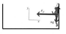
An amusement park ride ( Chabay & Sherwood, 2002, p.106): There is an amusement park ride that some people love and others hate where a bunch of people stand against the wall of a cylindrical room of radius R, and the room starts to rotate at higher and higher angular speed ω (Figure 1). When a certain critical angular speed is reached, the floor drops away, leaving the people stuck against the whirling wall. Explain why the people stick to the wall without falling down. Include a carefully labeled force diagram of a person, and discuss how the person’s momentum changes, and why.
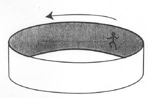
Figure 1.amusement park ride (Chabay & Sherwood, 2002, p.106)
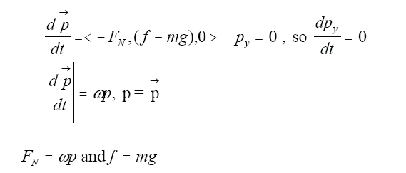
Figure 2. Physics diagram of the person (Chabay & Sherwood, 2002, p.106)
Starting from a fundamental physics principle, which is the momentum principle in this situation, we can determine the known forces and draw the force diagram (Figure 2). In the diagram, the person who has a mass m when the person is at the right, moving in the –z direction. The earth exerts a force which is mg downward. The wall exerts a force which has a y component +f because the person is not falling, and x component -FN normal to the wall because the person’s momentum is changing direction. There is momentum change. Since the net force is not zero, the person is not moving in a straight line. From circular motion (no change in y direction), and the momentum principle,
Combining these two,
The vertical component f of wall force is a frictional force. If the wall has friction which is too low, the person will not stick to the wall. So, f ≦ μFN (μ is the coefficient of friction). μ has a value which ranges between 0.1 to 1.0. The angular speed should be enough large. Thus,
. The smaller the friction, the higher the angular speed that is needed. When the frictional force is smaller than the gravitational force, people cannot stick to the wall and slide down. For this reason, the angular speed has to be large enough to make the frictional force greater than the gravitational force.
In this course, students write computer simulation programs to simulate physical systems using the VPython (Scherer, Dubois, & Sherwood, 2000). The VPython computer simulation program is suitable for Chabay & Sherwood’s curriculum because students do not need to have a programming background. Chabay & Sherwood (1999) explain why the VPython computer simulation program is suitable for this type of learning environment:
It is desirable that students themselves write the computer programs so that there are no impenetrable “black boxes.”…It is also desirable that students produce 3-D animations of physical systems, and electric and magnetic fields, not just graphs, but in standard programming environments this has been very difficult to do, and students in the introductory calculus-based physics course are very knowledgeable about all uses of computers save one: programming…There isn’t time to teach programming, much less how to do 3-D graphs, so it is essential to have a suitable programming environment that needs little instruction. VPython provides a suitable environment for the purpose (p.11-12).
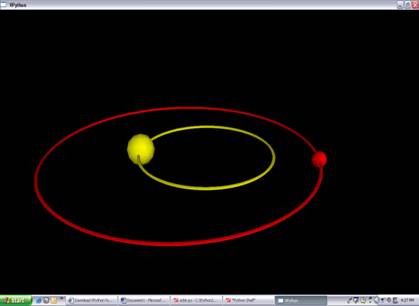
David Scherer (Scherer et al., 2000), a student in the Matter & Interactions course at Carnegie Mellon, created VPython in 2000. The VPython program requires that students focus on physics computations to get 3-D visualizations. The VPython supports standard vector estimates, so students can represent calculations in vector form. In other words, students can do true vector estimates, which improves their understanding of the utility of vectors and vector notation. For example, students can study the motion of the earth in orbit around the sun as writing a program by VPython. The printout of the simulation is shown in Figure 1.
Figure 3. Visualization for the VPython planetary orbits (Ornek, 2008).
Figure 3 shows that a planet with a mass of ½ that of the sun is orbiting the sun in a nearly circular orbit while the sun does its orbit. While students write their own computer simulation programs and can vary the mass of the sun and the mass of planet, they need to cope with physics. Thus, Students can understand how the gravitational force law,
works between the Sun and the Earth, and how the momentum principle,
works (G is the universal gravitation constant, m1, m2 represent the masses of two objects—here is the masses of the Earth and the Sun and is the distance separating the objects centers. This is a nice example of complex behavior emerging form simple physics principles, in this case the momentum principle and the gravitational force law. This illustrates the power of fundamental physics principles and gives a graphic example of the time evolution character of the momentum principle (Ornek, 2008). An example is shown in Table 1.
Table 1. VPython Program for Producing a Real-Time 3-D Animation in Figure 1 of the Earth Going in Orbit around the Sun (Ornek, 2008).
- from visual import *
- sun = sphere()
- sun.pos = vector(-1e11,0,0)
- sun.radius = 2e10
- sun.color = color.yellow
- sun.mass = 2e30
- sun.p = vector(0, 0, -1e4) * sun.mass [initial momentum of the sun]
- earth = sphere()
- earth.pos = vector(1.5e11,0,0)
- earth.radius = 1e10
- earth.color = color.red
- earth.mass = 1e30
- earth.p = -sun.p
- for a in [sun, earth]:
- a.orbit = curve(color=a.color, radius = 2e9)
- dt = 86400
- while 1:
- rate(100)
- dist = earth.pos - sun.pos [distance between the earth and the sun]
- force = 6.7e-11 * sun.mass * earth.mass * dist / mag(dist)**3 [the gravitational force law between the sun and the earth]
- sun.p = sun.p + force*dt [updating the momentum for the sun]
- earth.p = earth.p - force*dt [updating the momentum for the earth]
- for a in [sun, earth]:
- a.pos = a.pos + a.p/a.mass * dt
- a.orbit.append(pos=a.pos)
Note: The explanations in [ ] are physics relationships that must be set by students. Setting up these physics relationships is the model-building step. According to Chabay & Sherwood (2002), the modeling-based interactive engagement method can offer the potential to promote conceptual understanding of physics. Ornek (2007) found that the modeling-based interactive engagement teaching method enhances students to improve their understanding and construction of physics knowledge. In the study of Ornek, Robinson, & Haugan (2008), it was found that students at Purdue University in the US have closer views with most scientists (more favorable views) at the beginning of the course and at the end of the course than students at other universities. That finding suggests that students’ expectations, attitudes, and beliefs about a physics course based on modeling and interactive engagement are more sophisticated and professional than those of students in other physics courses at other universities. Hence, we wanted to investigate how this teaching method promotes students’ problem-solving ability and whether they act like experts while they are solving physics problems.
Purpose of the study and research questions
The purpose of this study was to investigate students’ performance on physics problem solving. The focus of the study was:
- How does the interactive-engagement modeling-based teaching approach promote students’ problem solving ability?
- Do students act like experts while they solve physics problems?